1. Introduction
This is an article about NumPy in Python. Numpy is a numerical python library. You can use it for array processing and operate on multidimensional arrays. You can do mathematical and logical operations.
2. Python Numpy
2.1 Prerequisites
Python 3.6.8 is required on windows or any operating system. Pycharm is needed for python programming. Numpy 1.20.3 needs to be installed.
2.2 Download
Python 3.6.8 can be downloaded from the website. Pycharm is available at this link.
2.3 Setup
2.3.1 Python Setup
To install python, the download package or executable needs to be executed.
2.3.2 Numpy Setup
You can install lumpy by using the command below:
Numpy installation
pip3 install numpy==1.20.3
2.4 IDE
2.4.1 Pycharm Setup
Pycharm package or installable needs to be executed to install Pycharm.
2.5 Launching IDE
2.5.1 Pycharm
Launch the Pycharm and start creating a pure python project named HelloWorld. The screen shows the project creation.

The project settings are set in the next screen as shown below.

Pycharm welcome screen comes up shows the progress as indicated below.

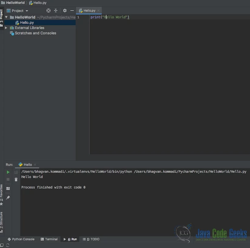
You can create a Hello.py and execute the python file by selecting the Run menu.
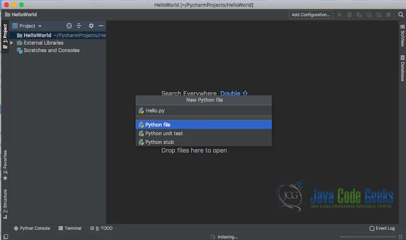
The output message “Hello World” is printed when the python file is Run.
2.6 What is NumPy?
Numpy is an open-source python package that has a set of routines for array processing. It was created by Jim Hugunin. It was called Numeric. Numarray was developed later. Numpy name was given by Travis Oliphant in 2005 by merging Numeric and Numarray.
2.7 Why Use NumPy?
You can use Numpy for array processing, mathematical/logical operations on arrays, Fourier transforms, share manipulation, linear algebra operations, and random number generation. You can use Scipy and Matplotlib with Numpy for scientific data analysis and plotting.
2.8 Why is NumPy Faster Than Lists?
Numpy arrays are memory-based and you can have similar data types in an array. A list in python can handle different data types which is the problem for computation. Numpy is five times faster than the lists in python. Numpy performs better as the data structures consume less space. Scipy and Numpy linear algebra functions are optimized for performance. N-dimensional properties help in making Numpy arrays perform. There are scenarios where lists are faster than Numpy arrays when data is appended. Appending data in the case of lists is the order of 1 O(1) and in Numpy, it is O(n).
2.9 Array creation
In NumPy, an array can be created by using an empty function specifying the dimensions (shape) and the data type. you can also create by using the array function by specifying the array. The sample code is shown below.
Numpy Array
import numpy as np
empty_array = np.empty([4,3], dtype = int)
print(empty_array)

list_1= [2, 4, 6, 8]
nd_array = np.array(list_1)
print (nd_array)

numbers = np.array([
       [1, 2, 3],
        [4, 5, 6],
        [6, 7, 9],
    ])

print(numbers)
You can execute the above code using the command below:
Array Creation Code Compilation
python3 array_creation.py
The output of the code executed is shown below:
Array Creation Output
apples-MacBook-Air:python_numpy bhagvan.kommadi$ python3 array_creation.py
[[-9223372036854775808 -9223372036854775808  4616981938510757901]
 [ 4613349226564724111 -9223372036854775808 -9223372036854775808]
 [ 4612217596255076360  4612217596255138984  4612217596255138984]
 [     924846352049320  4616981938510815294  4613349226564724111]]
[2 4 6 8]
[[1 2 3]
 [4 5 6]
 [6 7 9]]
2.10 Array Indexing
In NumPy, indexing is done like in python. Indices can be positive or negative based on the current position in the array. Colon is used to accessing the rest or all. Two colons are used to skip elements. Indexing can be done by using commas between axes. Multiple axes can be indexed by using a set of square brackets. The code below shows how indexing of arrays is done.
Array Indexing
import numpy as np
nd_array = np.array([
      [16, 31, 2, 13],
       [15, 10, 11, 8],
       [91, 6, 7, 12],
   [41, 15, 14, 12]
   ])

for i in range(4):
        print("row sum", nd_array[:, i].sum())
        print("column sum",nd_array[i, :].sum())
You can execute the above code using the command below:
Array Indexing Code Compilation
python3 array_indexing.py
The output of the code executed is shown below:
Array Indexing Output
apples-MacBook-Air:python_numpy bhagvan.kommadi$ python3 array_indexing.py
row sum 163
column sum 62
row sum 62
column sum 44
row sum 34
column sum 116
row sum 45
column sum 82
2.11 Basic operations
Index-based selection is great, but what if you want to filter your data based on more complicated nonuniform or nonsequential criteria? This is where the concept of a mask comes into play.
A mask is an array that has the exact same shape as your data, but instead of your values, it holds Boolean values: either True or False. You can use this mask array to index into your data array in nonlinear and complex ways. It will return all of the elements where the Boolean array has a True value.
Let us first see how masks and filters are used in bumpy. A mask is like an array that has the shape of the array and boolean values. You can see the code below how masks and filters are used.
Mask and Filter
import numpy as np
nd_array = np.linspace(4, 50, 24, dtype=int).reshape(4, -1)
print(nd_array)
mask_div_3 = nd_array % 3 == 0
print("mask divisible by 3",mask_div_3)
print(nd_array[mask_div_3])
divisible_by_3 = nd_array[nd_array % 3 == 0]
print("filtered divisible by 3",divisible_by_3)
You can execute the above code using the command below:
Mask Filter Code Compilation
python3 mask_filter.py
The output of the code executed is shown below:
Mask Filter Output
apples-MacBook-Air:python_numpy bhagvan.kommadi$ python3 mask_filter.py
[[ 4  6  8 10 12 14]
 [16 18 20 22 24 26]
 [28 30 32 34 36 38]
 [40 42 44 46 48 50]]
mask divisible by 3 [[False  True False False  True False]
 [False  True False False  True False]
 [False  True False False  True False]
 [False  True False False  True False]]
[ 6 12 18 24 30 36 42 48]
filtered divisible by 3 [ 6 12 18 24 30 36 42 48]
Now let us look at array transposing. Below is the example shown in code:
Transpose
import numpy as np
nd_array = np.array([
      [1, 12],
      [4, 14],
       [7, 16],
   ])
print(nd_array.T)
print(nd_array.transpose())
You can execute the above code using the command below:
Transpose Code Compilation
python3 transpose.py
The output of the code executed is shown below:
Transpose Code Execution Output
apples-MacBook-Air:python_numpy bhagvan.kommadi$ python3 transpose.py
[[ 1  4  7]
 [12 14 16]]
[[ 1  4  7]
 [12 14 16]]
apples-MacBook-Air:python_numpy bhagvan.kommadi$
Now let us look at array sorting. Sample code is attached below:
Array Sorting
import numpy as np
nd_array = np.array([
 [6, 1, 4],
       [9, 7, 3],
    [12, 2, 5]
    ])
print("sorting the array",np.sort(nd_array))
print("sorting the array with no axis",np.sort(nd_array, axis=None))
print("sorting the array using axis 0",np.sort(nd_array, axis=0))
You can execute the above code using the command below:
Array Sorting Code Compilation
python3 array_sorting.py
The output of the code executed is shown below:
Array Sorting Code Execution Output
apples-MacBook-Air:python_numpy bhagvan.kommadi$ python3 array_sort.py
sorting the array [[ 1  4  6]
 [ 3  7  9]
 [ 2  5 12]]
sorting the array with no axis [ 1  2  3  4  5  6  7  9 12]
sorting the array using axis 0 [[ 6  1  3]
 [ 9  2  4]
 [12  7  5]]
apples-MacBook-Air:python_numpy bhagvan.kommadi$
Now let us look at concatenate function. The same code is shown below :
Array Concatenation
import numpy as np
nd_array1 = np.array([
       [5, 9],
      [16, 10]
    ])
nd_array2 = np.array([
      [13, 15],
       [71, 27],
    ])

print("hstack",np.hstack((nd_array1, nd_array2)))
print("vstack",np.vstack((nd_array2, nd_array1)))
print("concatenate",np.concatenate((nd_array1, nd_array2)))
print("concatenate with no axis",np.concatenate((nd_array1, nd_array2), axis=None))
You can execute the above code using the command below:
Array Concatenation Code Compilation
python3 array_concatenate.py
The output of the code executed is shown below:
Array Concatenation Code Execution Output
apples-MacBook-Air:python_numpy bhagvan.kommadi$ python3 array_concatenate.py
hstack [[ 5  9 13 15]
 [16 10 71 27]]
vstack [[13 15]
 [71 27]
 [ 5  9]
 [16 10]]
concatenate [[ 5  9]
 [16 10]
 [13 15]
 [71 27]]
concatenate with no axis [ 5  9 16 10 13 15 71 27]
apples-MacBook-Air:python_numpy bhagvan.kommadi$
Aggregation functions are related to the sum, mean, max, the standard deviation of arrays.
2.12 Unary operators
Now let us look at unary functions which are sum, subtract, multiply, divide, exponential, add.reduce, and sum. Below is the sample code which shows the unary operators.
Array Creation Output
import numpy as np
nd_array1 = np.arange(16, dtype = np.float_).reshape(4,4)

print('First array:', nd_array1)

nd_array2 = np.array([12,12,12,12])
print('Second array:',nd_array2)

print('Add the two arrays:',np.add(nd_array1,nd_array2) )

print('Subtract the two arrays:',np.subtract(nd_array1,nd_array2))

print('Multiply the two arrays:' ,np.multiply(nd_array1,nd_array2) )

print('Divide the two arrays:',np.divide(nd_array1,nd_array2))
You can execute the above code using the command below:
Unary Operations Code Compilation
python3 unary_operations.py
The output of the code executed is shown below:
unary_operations Output
apples-MacBook-Air:python_numpy bhagvan.kommadi$ python3 unary_operators.py
First array: [[ 0.  1.  2.  3.]
 [ 4.  5.  6.  7.]
 [ 8.  9. 10. 11.]
 [12. 13. 14. 15.]]
Second array: [12 12 12 12]
Add the two arrays: [[12. 13. 14. 15.]
 [16. 17. 18. 19.]
 [20. 21. 22. 23.]
 [24. 25. 26. 27.]]
Subtract the two arrays: [[-12. -11. -10.  -9.]
 [ -8.  -7.  -6.  -5.]
 [ -4.  -3.  -2.  -1.]
 [  0.   1.   2.   3.]]
Multiply the two arrays: [[  0.  12.  24.  36.]
 [ 48.  60.  72.  84.]
 [ 96. 108. 120. 132.]
 [144. 156. 168. 180.]]
Divide the two arrays: [[0.         0.08333333 0.16666667 0.25      ]
 [0.33333333 0.41666667 0.5        0.58333333]
 [0.66666667 0.75       0.83333333 0.91666667]
 [1.         1.08333333 1.16666667 1.25      ]]
apples-MacBook-Air:python_numpy bhagvan.kommadi$
3. Download the Source Code
You can download the full source code of this example here: Python Numpy Tutorial